CAD for synthetic-biology binding networks

Biocircuits Explorer

The design workbench for binding-network engineers. Sketch reactions, verify the response geometry your circuit can reach, and commit to the design that survives parameter drift — all on one canvas, before a single primer is ordered.

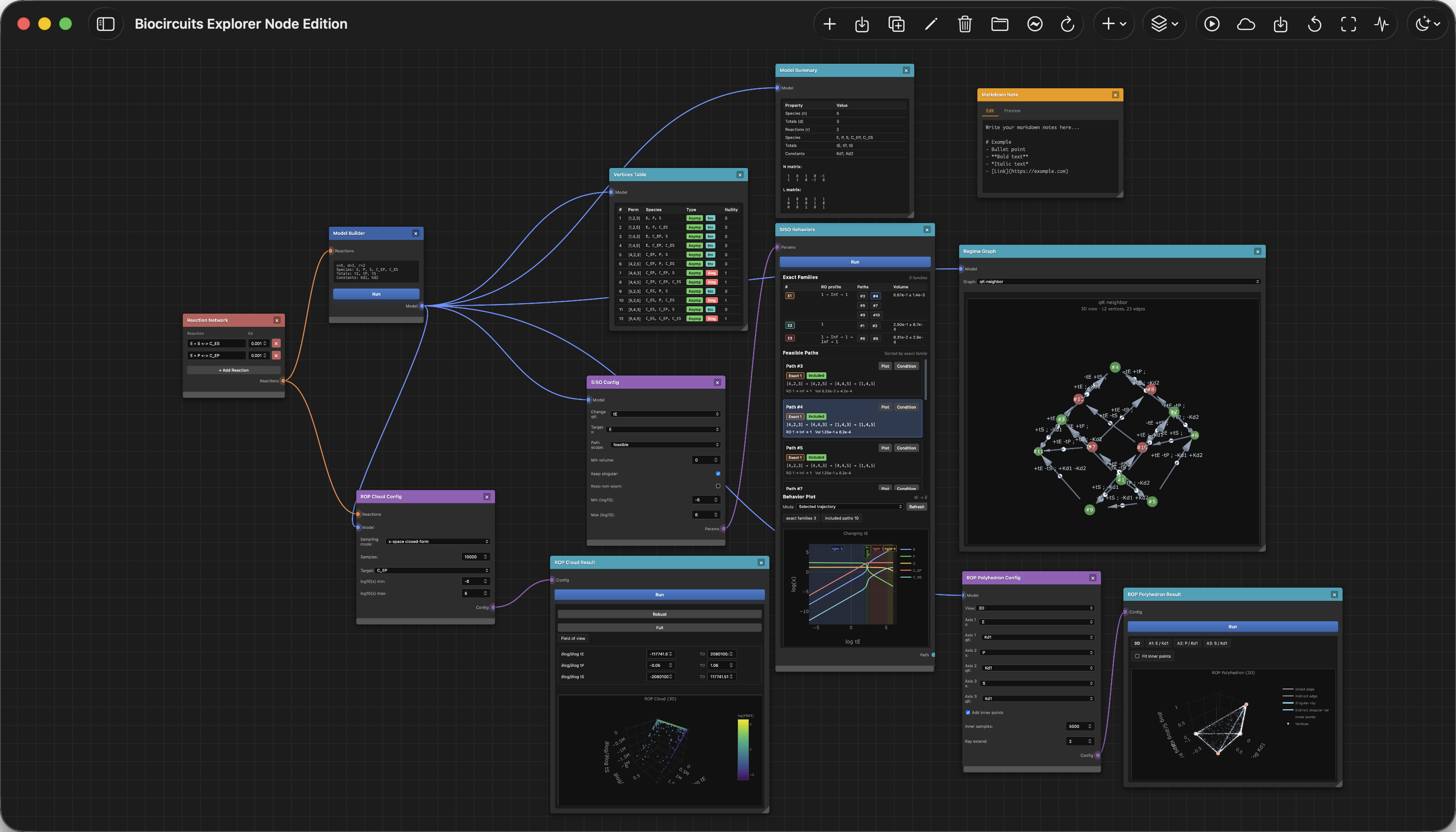
Biocircuits Explorer workbench overview

Reaction sketch in. Verified response surface out.

Hardware CAD let chip designers stop fabricating prototypes to find out what their circuit would do. Biocircuits Explorer does the same for binding networks: the polyhedron of every regime your circuit can occupy is computed up front, so you commit to the design that survives parameter drift — not the one that happened to work in the last experiment.

Same workspace model. Three ways to run it.

Deploy to a browser, install the native macOS app, or stay on the original form UI for scripted work. Workspaces and atlas libraries are portable JSON across all three.

Web

Biocircuits Web

The full design canvas, served from any modern browser. Best for teams behind a shared backend, classroom deployments, and remote collaborators on a managed server.

  • Full node canvas with zero install
  • Cloud Compute for long-running atlas builds
  • Cognito-backed accounts and per-user quotas
Open web app
macOS

Biocircuits for macOS

SwiftUI shell with an on-device project drawer and an app-managed backend. Best for individual designers who want workspace files on disk and an atlas library that never leaves the machine.

  • Local project drawer and document files
  • App-managed Julia backend
  • SQLite atlas libraries on disk
Release downloads
Classic

Classic form UI

The original form-based interface, kept around for reproducible scripting, headless reruns, and benchmarking against the canvas workflow.

  • Direct form-based parameter entry
  • Compatible with existing notebooks and scripts
  • Useful for headless reproduction
Open classic UI

Five primitives. One design surface.

Each primitive is a live node on the canvas. Wire them up, run, and the workspace updates in place — the same iteration loop a hardware designer expects from EDA.

01 · Response-surface geometry

The polyhedron of every regime your circuit can occupy.

Enumerate the exact vertices, edges, and faces of the Reaction Order Polyhedron. Rotate the geometry, inspect supports, and read dominant orders directly off the surface — the same way an EDA tool exposes timing margin instead of a binary yes/no.

  • Exact vertex and face enumeration
  • Interactive 3D rotation and inspection
  • Dominant order labels per vertex

02 · Input-output verification

What the circuit will actually do between regimes.

Walk the SISO paths your input/output pair traces as parameters change. Compare asymptotic and singular families side by side. Spot the regimes a circuit will live in, before a single wet-lab cycle confirms it.

  • SISO path traversal with regime overlays
  • Asymptotic vs. singular family comparison
  • Behavior signatures pinned to inputs and outputs

03 · Tolerance analysis

Sweep parameters before the bench commits to them.

Run 1D and 2D parameter scans with live plotting. Pin a crosshair, drag across the grid, and the result node updates without leaving the canvas. The same tolerance loop a board designer runs against component variance — except the variance here is biology.

  • 1D and 2D scans with live plotting
  • Interactive crosshair and value readout
  • Results feed straight back into downstream nodes

04 · Robustness under noise

Which regimes survive in the parameter cloud?

Sample parameter space stochastically and overlay the cloud onto the polyhedron. Robust regimes show up as dense clusters; fragile ones are sparse outliers. Pick the design that lands in a robust regime under cell-to-cell variation — not just the one that looks clean on the schematic.

  • Stochastic sampling across parameter space
  • Point cloud overlaid on polyhedron geometry
  • Volume-fraction robustness score per regime

05 · Inverse design, AI Import, remote compute

The library, the agent, and the cluster.

Atlas-backed inverse design searches a library for networks that realize a target behavior. AI Import turns a paper or notebook into a populated analysis chain in one click. Cloud Compute offloads heavy atlas builds to AWS Batch. Workspaces stay versionable JSON across all of it.

  • Atlas inverse design with motif, witness, and robustness queries
  • AI Import via Claude or DeepSeek (key stays in your browser)
  • Cloud Compute with Cognito accounts and per-user quotas

From hypothesis to a design you can defend in review.

Four steps that follow the same path in the browser, the native macOS shell, or the classic form UI. Workspaces and atlas libraries stay portable between them.

  1. Sketch the binding network

    Type the reactions, Kd values, conserved totals, and observable species — or have AI Import extract them from a paper in one pass.

  2. Compile the symbolic model

    The model-builder turns the sketch into the matrices N and L, enumerates the regime vertices, and hands you a session every downstream node reuses.

  3. Verify response geometry

    Walk SISO paths, run parameter scans, sample the parameter cloud, and search the atlas. Exercise every regime your circuit can reach before you commit to a build.

  4. Ship the design

    Export the workspace as portable JSON, hand off SQLite atlas libraries, and reproduce the same analysis on a teammate's machine — or on a CI worker.

Start designing biocircuits.

Open the web app for instant access, or install the macOS app for on-device projects and an app-managed backend. Both ship with the full canvas.

Web version

Open the canvas in your browser.

Zero install. Best for shared deployments, classroom sessions, and reviewing teammates' workspaces against a managed backend.

Open Web App

macOS version

Run the design loop on your Mac.

SwiftUI shell with an on-device project drawer, document files, and an app-managed Julia backend. Packaged builds ship through GitHub Releases.