Wiki · Chapter 1
Introduction to Reaction Order Polyhedra and the Biocircuits Explorer workbench
A practical guide to the mathematical objects behind the polyhedron, the nodes shown on the canvas, and the workflow that turns a binding network into a checkable analysis.
1What this wiki is
Biocircuits Explorer is a workbench for analysing equilibrium binding networks through the lens of Reaction Order Polyhedra (ROP). The homepage shows the entry points; this wiki goes one level deeper. It explains the mathematics the app is computing, the names of the geometric objects on the canvas, and the practical recipes that turn a circuit question into a reproducible analysis step.
Read it linearly the first time. Once you have built a few networks, each chapter section is meant to stand on its own as a reference.
Who this is for
New users of the web or macOS app who want to know what the regime graphs, SISO paths and polyhedra are actually showing them — not just how to click the buttons. No prior background in algebraic geometry or chemical reaction network theory is assumed; basic equilibrium thermodynamics (mass action, conserved totals) is.
Reading scope
This is not a promise of a stable external API. Node names, buttons, and cloud-deployment details describe the current repository. The theory sections describe asymptotic structure for equilibrium binding networks; numerical conclusions still need to be checked over the parameter ranges you plan to use.
2Theory of Reaction Order Polyhedra
2.1What is a Reaction Order Polyhedron?
A Reaction Order Polyhedron is a geometric object that organizes the asymptotic regimes an equilibrium binding network can enter at different parameter scales. It does not replace numerical parameter choices; it gives you a structural map before you start scanning them.
The input to an ROP analysis is a binding network:
- A finite set of base species \( X_{1}, \ldots, X_{n} \).
- A finite set of complexes — stoichiometric combinations such as \(AB\), \(AAB\), \(ABCD\). A complex is an integer vector \( a \in \mathbb{N}^{d} \setminus \{0\}\) with size \( |a|_{1} = \sum_{i} a_{i} \le \mu \), where \(\mu\) is the maximum allowed complex size.
- A finite set of reversible association reactions \( C_{a} + C_{b} \rightleftharpoons C_{a+b} \) with equilibrium constants.
- A stoichiometry matrix \(N\) (rows are reactions) and a conservation-law matrix \(L\) whose rows encode the conserved totals \( q_{i} = \sum_{j} L_{ij}\,x_{j} \).
- A choice of which totals act as inputs \(u\), which are fixed conserved totals \(q\), and which complex concentration plays the role of the output \(y\).
What comes out is usually not a single equilibrium curve but a polyhedral structure in log-concentration / log-parameter space. A vertex corresponds to a complete asymptotic regime: the dominant species in each conserved pool has been fixed. Faces and edges record ties or switches between dominant terms, which become transitions between regimes.
The geometry is polyhedral because the equilibrium equations
\[ N \log x \;=\; \log k, \qquad L\,x \;=\; q \]are non-linear in concentrations but split into log-linear regions in the asymptotic limit. When one term dominates each total, species concentrations are approximated by monomials, and the output becomes a linear function of the log-parameters. The polyhedron maps which monomial wins where; unlike a single numerical curve, it also shows how parameter space is divided into regimes.
2.2Why dominance, why log-log?
At chemical equilibrium, every species concentration is determined by mass action plus conservation. Each conserved total is a sum of monomials in the free concentrations of the base species:
\[ q_{i} \;=\; \sum_{j \,:\, L_{ij} > 0} L_{ij}\, x_{j}. \]For the simplest example \( A + B \rightleftharpoons AB \) with \( K = [AB] / ([A]\,[B]) \), the total of \(A\) is a sum of two monomials in the free concentrations \([A]\) and \([B]\):
\[ q_{A} \;=\; [A] + [AB] \;=\; [A] + K\,[A]\,[B]. \]The central observation behind ROP is that away from switching boundaries, these sums usually have one dominant monomial. Moving in log-concentration space crosses boundaries where that dominant term changes. Inside one regime, the dominant approximation gives power-law relationships among concentrations.
In log-log coordinates this relationship is easier to read. If the output \(y\) and input \(u\) satisfy \( y \asymp C\,u^{\rho} \) in some regime, then \( \log y = \rho \log u + \mathrm{const.} \) The slope is exactly the reaction order:
\[ \rho \;=\; \frac{\partial \log y}{\partial \log u}. \]Two facts make this useful:
- Within a regime, \( \rho \) is an integer (or a simple rational arising from stoichiometry), because the dominating monomial is a single product of integer powers.
- Across a one-dimensional input scan, the response is piecewise linear in log-log: a sequence of straight segments with integer slopes, joined at turning points where one monomial overtakes another.
A chosen one-dimensional input scan can therefore be summarized by a finite program of reaction orders:
\[ b \;=\; (\rho_{1}, \rho_{2}, \ldots, \rho_{L}), \quad\text{for example}\quad 0 \to -1 \to +1 \to 0 \to -2. \]Each entry is a slope; each transition is a turning point on the polyhedron. For multi-input / multi-output slices the analogous object is a sequence of gain matrices \( G_{\ell} = \partial \log y / \partial \log u \).
2.3The objects on the polyhedron
Biocircuits Explorer mostly follows the vocabulary used in the ROP papers. Some of these objects appear directly on the canvas; others are the computation behind result tables and plots.
- Reaction-order matrix
- The Jacobian of \(\log x\) with respect to \(\log(q, k)\). Its entries are the local reaction orders. Vertices, faces and the polyhedron itself are organized around how this matrix changes.
- Assignment
- A choice of one dominating species per conserved total: in pool \(i\), species \(j\) holds (almost) all the mass.
- Assignment polytope \(\mathrm{AssignP}(L)\)
- The convex hull of every legal assignment — a coarse outer envelope, the Cartesian product of one simplex per total.
- Dominance regime
- An assignment that is actually realizable by some \( x \in \mathbb{R}^{n}_{>0} \). Some assignments are spurious; only the realizable ones are real regimes.
- Dominance polytope \(\mathrm{DomP}(L)\)
- The convex hull of the dominance regimes. This is the tight polyhedral envelope of the dominance modes \( A(x) = \Lambda_{Lx}^{-1} L\, \Lambda_{x} \). Every vertex is an achievable regime.
- Vertices · faces · edges
- Vertices = complete asymptotic regimes (one winner per total). Faces = partial regimes with ties between several species. Edges = one-step transitions where a tie resolves. Walking around the polytope is walking through the regimes a real circuit visits as parameters change.
- Supports
- The set of monomial terms that survive in a given regime. Supports change from vertex to vertex.
- Input/output projection
- Choosing a scanned input \(u\) and an output \(y\) projects the polyhedron onto the \((\log u, \log y)\) plane. The image is the SISO regime structure.
- SISO path
- The sequence of vertices the system visits as the scanned input is swept from \(0\) to \(\infty\). The reaction-order program \( b = (\rho_{1}, \ldots, \rho_{L}) \) reads off the slopes along that path.
- Asymptotic vs. singular regimes
-
Inside a vertex \( \rho \) is a finite integer. On certain faces it
can be infinite or undefined (vertical jumps in log-log). The app
keeps the distinction — singular tokens \(\pm \infty\) and
NaNare not collapsed into a finite reaction order. - Capability periodic table
- A two-coordinate index \((d, \mu)\) — the number of base species and the maximum complex size — where each cell corresponds to a finite search space. Cells carry a capability envelope: mechanisms realized, strength extrema, robustness extrema, minimal witness networks, and certificates of un-reachability.
- Sign words
- Run-length-compressed three-state programs over \(\{-, 0, +\}\). The zero state is real (saturation / invariance) and is preserved during sign compression. Mechanism classes include activation from zero \(0 \to +\), settling to zero \(+ \to 0\), direct reversal \(+ \to -\), and zero-mediated reversal \(+ \to 0 \to -\).
2.4What the polyhedron tells you about a circuit
Once the polyhedron is built and a SISO (or MIMO) projection is chosen, several practically useful objects fall out:
- Response orders. The slopes \(\rho_{\ell}\) along the SISO path are the local Hill-like exponents. A regime with \(\rho \approx 0\) is saturated; \(\rho \approx 1\) is linear; \(\rho > \mu\) is ultrasensitive relative to the maximum complex size.
- Sensitive vs. saturated regions. The polyhedron helps locate these regions in log-parameter space, often before doing a dense numerical sweep.
- Switching loci / turning points. Faces of the polyhedron — projected to the input axis — give the inputs at which qualitative behavior changes. A boundary has the affine log-space form \[ a_{u}\,\log u + a_{q}^{\top}\!\log q + a_{K}^{\top}\!\log K + c = 0, \] so a turning point sits at \[ \log u^{\ast} \;=\; -\,\frac{a_{q}^{\top}\!\log q + a_{K}^{\top}\!\log K + c}{a_{u}}. \] Whether a switch is controlled by binding constants, by conserved totals, or mixed, is a built-in mechanistic classification.
- Upper-bound reachability. Conservation gives \( x_{a} \le U_{a}(q) = \min_{\,i:\,a_{i}>0}\, q_{i}/a_{i} \). Whether the output's vertex sits at this bound tells you whether the circuit can be driven to its stoichiometric ceiling.
- Robust regions. A program may be strong but fragile, weak but robust, or both. The polyhedron provides the geometry used to compute volume-fraction robustness scores (R-index); the value still depends on the chosen parameter domain and filters.
- Achievable behavior families. Different mechanisms can produce the same regime graph and sign word; the periodic table groups them into classes (activation, repression, settling to zero, zero-mediated reversal, multi-turn programs, MIMO rank expansion). The atlas workflow searches this family space.
2.5A worked example: \(A + B \rightleftharpoons AB\)
Take the simplest non-trivial binding network, with equilibrium constant
\[ K \;=\; \frac{[AB]}{[A]\,[B]}, \qquad q_{A} = [A] + [AB], \qquad q_{B} = [B] + [AB]. \]Scan \(q_{A}\) as the input \(u\), hold \(q_{B}\) fixed, take \(y = [AB]\) as the output. The conservation matrix is
\[ L \;=\; \begin{bmatrix} 1 & 0 & 1 \\ 0 & 1 & 1 \end{bmatrix}, \]so each row of the dominance-mode matrix \(A(x)\) is a one-simplex: for the \(q_{A}\) row, mass sits somewhere between \(A\) and \(AB\); for the \(q_{B}\) row, between \(B\) and \(AB\). The four assignments are the four corners of the resulting square — and for this network all four are achievable, so the dominance polytope is the square. The vertices read:
- \((A, B)\): both species mostly free. \([AB] \approx K\,q_{A}\,q_{B}\), so \(\rho = 1\).
- \((AB, B)\): \(A\) is mostly bound, \(B\) mostly free. \([AB] \approx q_{A}\), so \(\rho = 1\) but the output is now hitting the \(A\) ceiling.
- \((A, AB)\): \(B\) mostly bound, \(A\) mostly free. \([AB] \approx q_{B}\), constant in \(u\), so \(\rho = 0\) — saturation.
- \((AB, AB)\): both totals collapse on the same complex; the limiting species switches between \(A\) and \(B\).
As \(u = q_{A}\) is increased, a SISO scan typically walks \( (A,B) \to (AB,B) \to (A,AB) \), reading off the reaction-order program
\[ \rho \,:\, 1 \to 1 \to 0, \]or, after run-length sign compression, a typical settling-to-zero response \( S(b) \,:\, + \to 0 \). Each vertex of the square is a regime; each edge is a turning point; the whole square is the dominance polytope for this circuit. Increasing \(\mu\) or \(d\) inflates the square into higher-dimensional polyhedra with richer vertex structure — the kind of design space the periodic table is built to chart.
3The canvas, in one minute
3.1Nodes, ports, wires
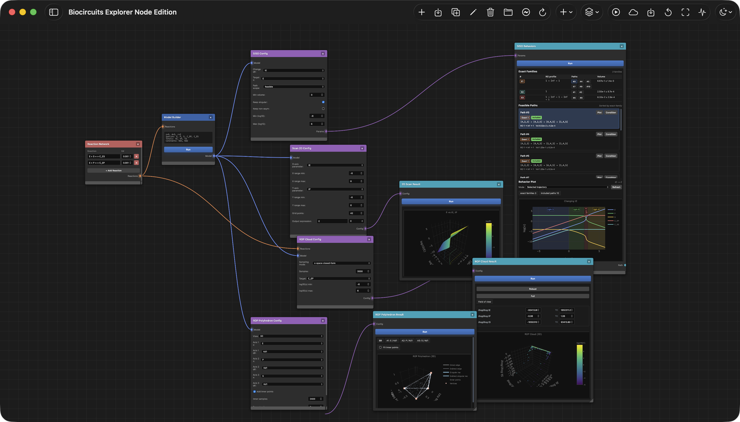
The web app opens to a blank canvas. You build an analysis by placing nodes and wiring their ports:
- Add a node. Click Add Node in the toolbar and choose from the categorized menu (Utilities, Input, Parameters, Process, Results).
- Connect ports. Each node has typed input sockets on the left and output sockets on the right. Click an output, drag to a matching input.
- Run. Most nodes have a Run button. The toolbar's Run Connected executes the whole connected subgraph in dependency order; Cloud Compute sends heavy work to a remote backend.
- Save. Save Workspace exports the whole canvas — nodes, parameters, wires — as portable JSON.
3.2Node families
The same five families recur:
- Input
-
reaction-networkfor hand-entered reactions;network-id-definitionto load a compressed network ID;sbml-importto bring in a model from an SBML file. - Process
-
model-builderturns reactions into a symbolic model (\(N\), \(L\), session ID).atlas-builderassembles a library of networks from an atlas spec.sbml-exportwrites a connected reaction source back out as SBML. - Parameters
-
siso-params,scan-1d-params,scan-2d-params,rop-cloud-params,rop-poly-params,fret-params,atlas-spec,atlas-query-config. - Results
-
model-summary,vertices-table,regime-graph,siso-result,qk-poly-result,scan-1d-result,scan-2d-result,rop-cloud-result,rop-poly-result,fret-result,atlas-query-result,atlas-inverse-result. - Utilities
-
markdown-notefor free-form notes you keep next to a workspace.
3.3Navigating & shortcuts
- Pan. Hold Space and drag, or drag with the middle / right mouse button, or scroll / two-finger swipe.
- Zoom. Ctrl/⌘ + scroll (or pinch on a trackpad).
- Select. Drag on empty canvas to rubber-band select; Shift+click a node to add/remove it. Drag any selected node to move the whole selection together.
- Align. With two or more nodes selected, an alignment toolbar appears (align edges/centers, distribute).
- Edit. Ctrl/⌘+Z undo, Ctrl/⌘+Shift+Z redo, Delete remove selection, Ctrl/⌘+A/C/V/D select-all / copy / paste / duplicate.
- Cheatsheet. Press ? any time for the full shortcut list; Esc clears the selection.
4Recipes — what to do, step by step
Each recipe below can be followed on its own. The flow line at the top of each one is the minimal node chain to build on the canvas.
4.1Build a model and inspect its regimes
Start here. This is the prerequisite for every other recipe.
-
Enter your reactions
Add a
reaction-networknode. For each reaction, type a line likeE + S <-> C_ESand a dissociation constantKd. Add as many lines as you need. -
Build the model
Wire
reaction-network→model-builder. Press Run. The builder fixes the symbolic order of species, complexes, totals and constants and returns a session ID downstream nodes will reuse. -
Inspect the model
Wire
model-builder→model-summaryto see \(n\), \(d\), \(r\), the species list, the totals, the binding-constant symbols, and the matrices \(N\) and \(L\). -
List the vertices
Add
vertices-tableoff the same model. Each row is a vertex of the polyhedron: its permutation of species, type (asymptotic vs. non-asymptotic), singular / invertible status, and nullity. -
See the regime graph
Add
regime-graph. The dropdown lets you switch between qK-neighbor (regimes joined by single parameter transitions) and SISO mode.
Reading the output
The vertices table is the discrete index of the polyhedron. The regime graph is its 1-skeleton. Together they tell you how rich the qualitative behavior of your network can be — before you have chosen a single number.
4.2Trace a SISO behavior path
Use this when you want to know how the circuit responds to changing one specific input.
-
Choose input, output and bounds
In
siso-paramspick the \(qK\) change variable (the swept input), the target species \(x\) (the output), the path scope (feasible, robust, or all), the minimum volume fraction, and the log\(_{10}\) bounds for the scan. -
Enumerate behavior families
Run
siso-result. The node returns a ranked list of SISO paths — each path is a reaction-order program \( b = (\rho_{1}, \ldots, \rho_{L}) \) with a feasibility volume. -
Visualise the chosen path
Click a path in the list. Wire to
qk-poly-resultto see the projected polyhedron in \(qK\)-space for that path.
Reading the slopes
The sequence of integers in a SISO path is the local log-log slope
at each step. If you see 0 → 1 → 0, it usually means
activation followed by saturation; 1 → 0 → −1 is
a non-monotone response with a peak. The signs alone, run-length
compressed, are the “sign word” the periodic table
indexes.
4.3Run a parameter scan
When you want a numerical response curve, not just the symbolic path.
-
Pick a parameter and a range
In
scan-1d-paramschoose a \(qK\) variable, the log range and number of points, and type an output expression — for example2*C_ES + E. -
Run and read
scan-1d-resultdraws the output expression versus the scanned variable. Crosshairs and value readouts feed downstream nodes. -
Go 2D when needed
Swap to
scan-2d-params/scan-2d-resultfor a heatmap across two parameters simultaneously.
4.4Visualize the ROP polyhedron and the point cloud
The polyhedron itself is one node; the point cloud sampled across parameter space is another. Together they help you spot candidate robust regions.
-
Configure the polyhedron view
In
rop-poly-paramschoose 2D or 3D, and pair each axis with a species \(x\) and a \(qK\) parameter. The inner sample count controls how the interior is filled in. -
Sample the cloud
rop-cloud-paramspicks the sampling mode (x-space or qK-based), the number of samples, the target species and the log-bounds. The result node plots the cloud overlaid on the polyhedron. -
Look for the dense regions
Vertices with a dense surrounding cloud are often more robust within the chosen sampling range and sampling mode. Sparse vertices are not automatically useless, but they do suggest a narrow parameter window.
4.5Atlas search and inverse design
The atlas workflow goes the other direction: given a behavior you want, find networks that may achieve it.
-
Specify the search space
atlas-spechas four tabs: Basic (source label, SQLite path, profile), Behavior (path scope, min volume), Enumeration (pairwise binding, reaction counts) and Explicit (JSON list of networks). -
Preview the library
Wire to
atlas-builderand click Build Preview — this generates a slice of the atlas so you can verify the spec before committing to a full build. -
Define the design goal
atlas-query-configlets you state the goal: an I/O pair (e.g.tA -> AB), a motif label, an exact behavior, a witness path, or forbidden regimes. Pick a ranking mode — minimal_first or robustness_first. -
Run forward or inverse
atlas-query-resultreturns the ranked match list.atlas-inverse-resultadditionally runs the build + query loop with negative-example refinement and returns candidates with evidence.
Heads up
The canvas builder is intended for previews and small
scratch atlases. For full-scale library construction use the CLI
scripts in webapp/build_atlas.jl and friends, then
point the query nodes at the resulting SQLite file.
5What it’s for — design applications
ROP analysis pays off in three broad situations:
- Reading off Hill-like exponents without curve-fitting. The integer slopes on the SISO path are asymptotic predictions for local response orders. Checking whether any regime has \( \rho > \mu \) is a first structural test for possible ultrasensitivity.
- Finding robust operating regimes. Point-cloud density is a sampling estimate of robustness: a vertex visited by many parameter samples is usually worth checking before a vertex that appears only in a narrow window.
- Inverse design. Given a target signal-processing behavior (a sign word, a target peak height, a robust settle-to-zero), the atlas tools enumerate binding networks that may realize it, ranked by minimality or robustness.
ROP analysis can also help explain why a circuit fails. If your target response is not in the polyhedron of any network in the periodic-table cell \((d, \mu)\) you searched, and that search space fully covers your modeling assumptions, the failure is more likely structural than numerical. The app reports this kind of negative evidence when it is available.
6How to read the outputs
A good ROP session is not just a stack of plots. The app is exposing several layers of evidence: a symbolic model, a finite list of regimes, an adjacency structure, asymptotic response orders, and numerical checks. This section gives a practical reading order.
6.1Regime table checklist
Start with model-summary and vertices-table.
They tell you whether the network you sketched became the network you
intended to analyze.
| Output field | What it means | What to check |
|---|---|---|
species, x_sym |
The species order used by the backend. | Make sure complexes such as AAB or C_ES are named consistently. |
q_sym, K_sym |
The conserved totals and binding constants that form the \(qK\) coordinate system. | These are the only variables a SISO scan can sweep directly. |
N |
The stoichiometry matrix for reaction constraints. | Unexpected rank or row count usually points to a malformed reaction list. |
L |
The conservation-law matrix. | Each row should match a conserved pool you can explain chemically. |
| Vertex type | Whether a regime is asymptotic, singular, invertible, or degenerate. | Finite response orders come from regular asymptotic vertices; singular entries need separate interpretation. |
| Nullity | The local degree of freedom left after the active constraints are imposed. | High nullity means the regime is underdetermined or lives on a larger face, not an isolated corner. |
If the model summary already looks wrong, do not proceed to SISO. Fix the reaction list first. A beautiful polyhedron for the wrong conserved pools is still the wrong answer.
6.2SISO interpretation checklist
A SISO result should be read at three levels: the exact slope program, the sign-compressed behavior, and the geometry that supports it.
| Pattern | Interpretation | Design question |
|---|---|---|
0 → + |
Activation from a flat baseline. | Can the output turn on only after the input crosses a boundary? |
+ → 0 |
Response that saturates. | Is the output ceiling set by a conserved total or by a binding constant? |
+ → - |
Direct reversal: increasing the input eventually represses the output. | Which complex steals the limiting species at the reversal? |
+ → 0 → - |
Zero-mediated reversal with a plateau. | Is the plateau robust enough to be a useful operating window? |
+ → 0 → + |
Two-stage activation separated by saturation. | Are there two independent binding thresholds? |
NaN or ±∞ |
Singular or vertical response in the projected coordinates. | Is this a meaningful jump, or did the chosen output vanish in that regime? |
The sign word is a summary, not the whole story. Two paths can share a sign word but differ in strength, vertex sequence, transition control, and robustness. Use the full slope list and the projected polyhedron before treating two behaviors as equivalent.
6.3Numerical scans versus asymptotics
The ROP polyhedron is an asymptotic object: it predicts which monomial dominates in wide log-parameter regions. Parameter scans are finite numerical evaluations. They should agree in the large-scale shape, but they answer different questions.
- Use SISO paths to learn which qualitative behaviors are structurally possible.
- Use parameter scans to check the finite constants you actually plan to use.
- Use ROP cloud to estimate which regimes occupy substantial parameter volume.
- Use atlas search when the current network cannot realize the behavior and you need candidate alternatives.
A useful rhythm
Build the model, read the vertices, choose an input and output, enumerate SISO paths, inspect the projected polyhedron, then run a numerical scan through the same coordinates. When these disagree, the disagreement is information: it usually points to a finite-size effect, a narrow transition, or an output expression that is not aligned with the asymptotic coordinate.
7Node reference
The canvas is a dataflow system. A node is useful when you know what it consumes, what it produces, and which backend endpoint it normally calls.
Model construction
reaction-network stores reactions and dissociation
constants. model-builder calls
/api/build_model and emits the session used by most
downstream analysis nodes.
Regime structure
model-summary, vertices-table, and
regime-graph expose the symbolic model, vertices, and
adjacency graph via /api/find_vertices and
/api/build_graph.
SISO analysis
siso-params defines the \(qK\) coordinate and output.
siso-result calls /api/siso_paths and
related endpoints; qk-poly-result renders selected
path geometry.
Scans and surfaces
scan-1d-result, scan-2d-result,
fret-result, rop-cloud-result, and
rop-poly-result turn a session into numerical curves,
heatmaps, sampled clouds, and polyhedron projections.
Atlas workflows
atlas-spec, atlas-builder,
atlas-query-config, atlas-query-result,
and atlas-inverse-result cover build, query, and
inverse-design workflows.
Interoperability
sbml-import parses an SBML file into editable
reactions via /api/v1/import/sbml (binding-network
subset; anything not representable is reported as warnings).
sbml-export writes a connected reaction source back
out via /api/v1/export/sbml.
Workspace notes
markdown-note has no backend dependency. It is there
so a saved workspace can carry assumptions, candidate mechanisms,
or why a particular path was accepted or rejected.
7.1Common wiring patterns
| Question | Minimum node chain | Typical next step |
|---|---|---|
| Did my reaction list parse correctly? | reaction-network → model-builder → model-summary |
Add vertices-table after the summary looks right. |
| What regimes exist? | model-builder → vertices-table |
Add regime-graph to inspect transitions. |
| How does one input affect one output? | model-builder → siso-params → siso-result |
Select a path and view it with qk-poly-result. |
| What curve will I see for one finite parameter set? | model-builder → scan-1d-params → scan-1d-result |
Compare the curve to the SISO slope program. |
| Which network can realize my target behavior? | atlas-spec → atlas-query-config → atlas-query-result |
Run atlas-inverse-result for build + query refinement. |
8Atlas and inverse design
The atlas layer turns many individual ROP analyses into a searchable design library. This is where the project stops being a single-model workbench and becomes a map of capability space.
8.1The four atlas objects
- Atlas spec
- The recipe for what to analyze: explicit networks, enumerated search spaces, behavior configuration, source labels, and optional SQLite persistence.
- Atlas
- A single build result. It usually contains network entries, behavior slices, and family buckets.
- Atlas library
- A stable aggregate assembled from one or more atlas builds. Use this when you want a versionable knowledge base.
- Atlas SQLite
- A persisted form for large or incremental libraries. Query nodes and CLI scripts can read from this directly.
8.2How to formulate a query
Good atlas queries are specific about both behavior and evidence. Start with an input/output pair, then add only the constraints that matter.
- Motif queries ask for broad classes such as activation, repression, reversal, or settling.
- Exact behavior queries ask for a specific slope list or sign word.
- Witness queries require a concrete path through vertices, not only a matching summary label.
- Forbidden-regime queries exclude circuits that visit undesirable intermediates.
- Robustness queries rank or filter by volume fraction rather than by existence alone.
8.3What inverse design returns
Inverse design is not just “search harder.” It combines build, query, negative knowledge, and candidate refinement. A useful result should tell you:
- which networks matched;
- which target kind was used (motif, exact behavior, witness, or support);
- whether a new atlas build or merge was performed;
- which candidates were rejected and why;
- whether the match is structurally exact or only a soft support match.
A failed inverse-design run can still be useful. If a whole \((d,\mu)\) cell fails an exact support screen, that is evidence that the desired behavior needs either more base species, larger complexes, or a different modeling assumption.
8.4Canvas versus CLI
Use the canvas while shaping the question. Use the CLI once the question is stable and the run becomes large.
julia --project=webapp webapp/build_atlas.jl spec.json atlas.json
julia --project=webapp webapp/query_atlas.jl atlas.json query.json result.json
julia --project=webapp webapp/run_inverse_design.jl spec.json inverse_result.json
The SQLite route is the right choice when you expect to reuse the library across many sessions or merge incremental builds over time.
8.5The Design Agent — describe a behavior, get a verified network
The Design Agent is the conversational front door to inverse design. You describe the dose–response behavior you want in plain language — in any language — and an LLM works with the live engine in the loop to find a network that actually produces it.
The division of labor matters, because it is what makes the answers trustworthy:
- The LLM is the planner, compiler, and critic. It reads your request, maps it to a standard behavior label, proposes a candidate network with binding constants, decides which engine tool to call next, and judges whether the result matches what you asked for.
- The Julia engine is the ground truth. For every candidate it builds the ODE model, solves it across a sweep of the input, and classifies the resulting shape. Nothing reaches you that was not actually simulated.
- The atlas is a seed and a prior, never a canned answer. The agent may retrieve a structurally similar network from the atlas to use as a starting point, then refine and re-verify it against the engine. It does not look up a stored result and hand it back.
The consequence is a hard honesty guarantee: the agent does not fabricate. If the compute engine is offline it tells you so instead of inventing a curve, and it will not turn a greeting or an off-topic message into a fake design. Check the status pill in the header — it reads Agent ready when the engine is reachable.
8.6Opening it and supplying an LLM key
Open the Design Agent view (the agent tab in the web app, or the agent page in the macOS app). To use free-form natural language you need an LLM key:
- Click the
⚙ LLM keybutton at the bottom-right. - Pick a provider — OpenAI-compatible (key + base URL) or Anthropic (x-api-key) — and paste your key. The optional base URL lets you point at a proxy or a compatible endpoint; the optional model field overrides the default.
-
Choose a reasoning effort. OpenAI exposes
low…xhigh; Anthropic maps to an extended-thinking budgetlow…max. Higher effort means more deliberate multi-step planning — better on hard 2D or ultrasensitive targets, at the cost of latency. - Click Save. Click anywhere outside the panel, or press Esc, to close it.
The key is kept only in this page's memory and is cleared on reload or close. It is sent only with each design request, which the backend forwards to the LLM you configured. Non-secret provider and model preferences remain in browser storage. Without a key a built-in keyword compiler still handles simple requests; a key unlocks arbitrary phrasing, including non-English.
8.7Worked examples
These are real prompts the agent handles. Phrase them however you like — the LLM maps your words to a standard label and the engine verifies the result.
- “A network whose target first falls, then rises as the input increases.”
- A biphasic valley. The agent seeds a structure, simulates the dose–response over the log-input window the engine itself chooses, and confirms the valley shape over the binding-constant prior.
- “monotone repression” / “output goes down as input goes up”
- A monotonically decreasing dose–response, verified by a 1D scan.
- “a bandpass — peak at intermediate input”
- An interior maximum; the agent locates the peak and reports where it sits.
- “an AND logic gate on two inputs”
-
A two-input request triggers a 2D scan. The agent checks that the four
corners of the input square booleanize to the AND truth table
(
[0,0,0,1]). - “a 2D heatmap with a single bright spot in the middle — as sharp as possible”
- A 2D ultrasensitive target. The agent runs a 2D scan, finds the interior peak, and reports its sharpness. Targets like this often benefit from a higher reasoning effort.
8.8Reading what comes back
- The reply
- A short natural-language answer comes first, explaining what was tried.
- Candidate cards
-
Each proposed network is shown as a clickable card: its reactions with
binding constants (
Kd) called out, the design rules, and a Top candidate plot of the engine-computed dose–response (or a heatmap, for 2D) with real axes, units, and the window the engine chose. Only a handful are shown, deduplicated by shape. Click a card to select it. - Evidence tier
- Every candidate carries how strongly it was checked — Tier 0 (prior only), Tier 1 (a single-Kd dose scan), or Tier 3b (sampled across the binding-constant prior). Higher tiers mean stronger verification.
- Export to Workspace
- Turns the selected candidate into a real reaction-network node on the canvas, so you can analyze it with the full ROP toolset (§4, §6).
- Saved with the project
- The conversation is stored per project, and every turn is recorded as a replayable trace — the tool calls plus engine results — so any result can be re-verified later against the live engine.
9AI Import — turn a paper into a model
The ai-import node turns clearly stated binding chemistry
from papers, supplementary material, or notebooks into a first draft.
It calls the language model you choose, tries to extract reversible
binding reactions, Kd values, and recommended downstream analyses, then
places editable nodes on the canvas. It reduces transcription work; it
is not a final modeling or literature-review authority.
Privacy posture
The project backend does not receive or store your API key. The browser sends it directly to the chosen provider. Tick “Remember for browser session” only if you trust the machine you are sitting at.
9.1What the node does
The node output is checked against a fixed schema and allow-list. It is allowed to:
-
Read pasted text, a PDF attachment, or a Jupyter
.ipynb(only source cells; outputs are stripped locally before the file is sent). - Emit one or more networks, each carrying a list of reversible binding reactions, a Kd in molar, and a confidence label.
- Pick recommended downstream analyses from a fixed allow-list. Anything else is dropped during post-processing.
- Add a warnings list for approximations, unit conversions, skipped files, or discarded models.
When you click Insert chain on a network card, the node
drops a reaction-network with the extracted reactions,
wires it into a model-builder, and adds one result
node per recommended analysis. Each spawned node is a normal canvas
node — edit reactions, change Kd values, rerun, save.
9.2Choosing a provider and supplying a key
The UI currently includes two provider choices, both called through the Anthropic Messages API shape:
| Provider | Models | Endpoint | Document attachments |
|---|---|---|---|
| Anthropic | Claude Opus 4.7, Sonnet 4.6, Haiku 4.5 | api.anthropic.com/v1/messages |
Yes (PDF) |
| DeepSeek | V4 Pro, V4 Flash (Anthropic-compatible) | api.deepseek.com/anthropic/v1/messages |
Text and notebook only |
Pick a model from the dropdown or type a custom model ID. The
provider is detected from the model name (anything starting with
claude goes to Anthropic, anything starting with
deepseek goes to DeepSeek). Actual model availability is
determined by the provider API; if a provider rejects PDF or document
blocks, use the text or notebook route. The API key field is a
password input; when “Remember for browser session” is unchecked,
the page does not write the key to sessionStorage.
9.3Inputs: text, PDF, notebook
The three input types can be used alone or combined; combined inputs are sent as one source packet:
- Text
- Paste a section, supplementary methods, abstract, anything relevant. Useful when you only want a few specific reactions out of a long paper.
-
Upload a paper. The whole PDF is sent as one
documentcontent block. Expect higher token usage than the text path. Only available on Anthropic models. - Notebook
-
Upload a
.ipynb. The browser parses it locally and sends only source cells (markdown + code). Output cells, base64 images and large data blobs never leave your machine.
9.4Reading the results and the auto-spawned chains
A finished run renders three things in the node body: a short paper summary, one card per extracted network, and a warnings list. Each network card carries an Insert chain button that materialises this on the canvas:
The recommended-results slot expands per network: a
model-summary is retained, plus zero or more of
vertices-table, regime-graph,
siso-result, scan-1d-result,
scan-2d-result, rop-cloud-result,
rop-poly-result, fret-result. Entries
outside this allow-list are dropped during post-processing and
reported as warnings.
9.5Validation rules — and what gets discarded
The prompt and post-processing constrain model output, but they do not guarantee correctness. Common handling rules:
-
Kd not stated. A placeholder
1e-3 Mis emitted, confidence is marked low, and the warning names the reaction. Topology survives; you must edit the value. - Only Ka given. The node emits \( K_{d} = 1 / K_{a} \) and notes the inversion in warnings.
- Only kon / koff. The node emits \( K_{d} = k_{\mathrm{off}} / k_{\mathrm{on}} \) and notes it.
- Hill functions, phenomenological dose-responses, catalytic turnover. Discarded with a warning. The node will not rewrite them as a binding scheme that was not stated.
- Unit conversion. nM / µM / mM are converted to M with a warning.
A run that returns zero networks plus a summary usually means the source does not contain extractable equilibrium binding chemistry, or that the provided material is insufficient for a structured reaction list. Add the relevant methods section, supplement, or reaction table rather than accepting a placeholder model.
10Accounts and sign-in
On a public deployment the cloud backend requires a signed-in user. On a local or on-prem deployment the sign-in button stays hidden and analysis requests run against the current in-process Julia backend without a project account.
10.1When you need to sign in
You need an account only for cloud-backed work:
- Submitting Cloud Compute jobs (atlas build, inverse design).
- Hitting per-user quotas — the daily submission counter is keyed by your Cognito user.
- Persisting result artifacts in the cloud backend's S3 prefix.
Local SISO analyses, regime graphs, point clouds, parameter scans, and model summaries work without an account. The toolbar's Sign in button only appears when the backend reports auth is enabled.
10.2The sign-in flow
Authentication uses AWS Cognito Hosted UI with the OAuth Authorization Code + PKCE flow:
-
Click Sign in in the toolbar
The button is hidden if Cognito is not configured. When it is, the SPA fetches
/api/auth/configto learn the Cognito domain and public app-client ID. -
Go through Cognito Hosted UI
The browser is redirected to
…amazoncognito.com/oauth2/authorize. Sign up or sign in there with email + password. Email verification and optional MFA are handled by Cognito. -
Bounce through
/auth-callback.htmlCognito redirects back to
/auth-callback.htmlwith an authorization code. The SPA exchanges the code for ID / access / refresh tokens using the PKCE verifier it stashed before redirect. -
Return to the app
The ID and refresh tokens are kept in this tab's
sessionStorage; the unused access token is discarded. The SPA then navigates back to the page that initiated sign-in. From this point every cloud job submission attachesAuthorization: Bearer <id_token>.
ID tokens auto-refresh five minutes before expiry using the
refresh token. Closing the browser tab or macOS app clears the session;
signing out clears it immediately and visits
Cognito's /logout endpoint so the next sign-in lands
on the Hosted UI fresh.
10.3Same flow on macOS
The Swift macOS app runs the same auth.js inside a
WKWebView. Authentication state is session-only and is
cleared when the app closes. It is not persisted in WebView
localStorage, and there is no native Keychain integration;
reopening the app therefore requires a new sign-in.
The Cognito app client must register the macOS WebView's loopback
callback (default http://127.0.0.1:18088/auth-callback.html)
alongside the web origin. See deploy/AWS_BATCH.md
§2.2 for the full callback-URL list.
10.4Per-user quotas
When the deployment opts in with --with-quota-table,
a DynamoDB counter is keyed by your Cognito sub.
Every cloud job submission writes to it; the counter resets via
a TTL field once per day.
The default daily limit is 50 jobs per user; the
operator can raise or lower it with
BIOCIRCUITS_EXPLORER_QUOTA_DAILY_LIMIT. Exceeding the
limit returns HTTP 429 from the cloud backend and no Batch
job is queued. Local analyses are not counted.
11Cloud Compute — running heavy jobs remotely
Two analyses can take minutes or hours: building a large atlas, and running inverse design over a large search cell. The Cloud Compute toggle redirects those jobs to a remote AWS Batch queue while keeping every other analysis on the in-process Julia backend.
11.1Toggling Cloud Compute
The toolbar has a Cloud Compute button that flips a
session-wide flag, persisted in localStorage:
- ON. Atlas builds and inverse-design runs are submitted as jobs to the cloud backend. The result node shows the job ID, a live status badge, and the link to the artifact when it finishes.
- OFF. The same nodes run their work locally and block the canvas while doing so. Fine for small previews.
Toggling Cloud Compute does not change the execution path for lightweight analyses in the current implementation (SISO paths, scans, polyhedron viewers). They still run on the local backend.
11.2Which jobs run remotely
| Endpoint | Route when Cloud Compute is ON | Route when OFF |
|---|---|---|
build_atlas |
AWS Batch job | Local Julia worker |
run_inverse_design |
AWS Batch job | Local Julia worker |
build_model, find_vertices,
siso_paths, parameter_scan_*,
rop_*, fret_*
|
Always local — the toggle is ignored. | |
11.3The deployment stack
On the operator side the cloud route uses four AWS surfaces. You do not need to know the details to use the app, but they matter when reading job logs or planning a deployment:
- ECR
-
Stores the worker Docker image. It is the same image as the
local backend, with a Batch entrypoint that reads
input.jsonfrom S3 and writesstatus.json/result.jsonback. - S3
-
One prefix per job, holding
input.json,status.json, andresult.json. The frontend pollsstatus.jsonand downloadsresult.jsonwhen the status becomes succeeded. - AWS Batch
-
Runs the worker image as a container in a managed compute
environment. Default
minvCpus=0so the cluster scales to zero between jobs. The job definition is registered with an execution role so ECR image pulls and CloudWatch log delivery work on both EC2-launch and Fargate-launch environments. - DynamoDB (optional)
-
Per-user daily submission counter keyed by Cognito
sub. Enabled with--with-quota-tableinsetup_aws_batch.sh. See §10.4 for the user-facing behaviour.
A signed Cognito ID token must accompany
POST /api/jobs requests when Cognito is configured.
The cloud backend rejects unsigned calls with
HTTP 400 “Missing Authorization Bearer token”.
For operators
The full setup script, IAM policy and callback-URL list live in
deploy/AWS_BATCH.md. It also covers the Cognito
integration and the DynamoDB quota table.
11.4Watching a remote job
The result node renders the job lifecycle inline:
- Job ID returned by Batch as soon as submission succeeds.
-
Status badge stepping through
pending → submitted → running → succeeded / failed /
            cancelled
. -
Result artifact linked when the run succeeds.
For atlas builds, the artifact is a SQLite file you can re-feed
into an
atlas-specnode on any future canvas session. - Error message from the worker when the run fails. Deeper logs live in CloudWatch under the Batch job's log group.
A job's full lifecycle — submission, queue, container start, run, result upload — is opaque from the canvas: you only see the status badge. If you need detail, the Batch console and the per-job S3 prefix are the right places to look.
12Troubleshooting and limits
Most confusing results come from one of three places: a reaction list that does not encode the intended chemistry, a stale model session, or an output expression that is not aligned with the chosen coordinate.
| Symptom | Likely cause | What to do |
|---|---|---|
Invalid session_id |
The backend restarted, the page was refreshed with stale nodes, or the session expired. | Run model-builder again, then rerun downstream nodes. |
| Unexpected species or missing complex | Reaction naming mismatch or malformed reaction syntax. | Check model-summary before running any result node. |
| No SISO paths returned | The selected \(qK\) coordinate/output pair has no feasible path under the current filters. | Relax path scope or volume thresholds; then try a different output species. |
| Scan curve disagrees with expected sign word | Finite constants are not deep enough in the asymptotic region, or the output expression mixes species. | Widen the log range and compare with the projected polyhedron. |
| Atlas query finds too many networks | The query describes only a broad motif. | Add an exact behavior, witness, forbidden-regime, or robustness constraint. |
| Atlas query finds nothing | The search cell, enumeration profile, or support condition is too restrictive. | Try a larger \((d,\mu)\) cell or inspect the negative evidence. |
12.1Modeling limits
The current workbench is built for equilibrium binding networks and conserved totals. It is not a general-purpose simulator for time-dependent kinetics, irreversible production/degradation, spatial transport, stochastic copy-number noise, or arbitrary ODE models. You can sometimes approximate those questions by choosing a steady-state binding subproblem, but that approximation should be stated explicitly.
The strongest answers are structural: possible / impossible behaviors, regime transitions, asymptotic slopes, and robustness in log-parameter space. Numerical scans are provided to connect that structure to finite parameter values, not to replace a full kinetic simulation when the biology demands one.
13Reference and further reading
For the formal development, see the papers in the repository:
-
Dominance polytope of binding networks — the long paper that
proves the polytope theorem (location:
doc/ROP_paper/). -
Capability periodic table for binding circuits — the short
paper that sets up the \((d, \mu)\) index, sign words, R-index
robustness, and minimal-witness machinery (location:
docs/rop_capability_periodic_table_paper_en.pdf). -
Periodic complete definition — implementation profile and
terminology bridge (location:
docs/periodic_complete_definition.md).
For practical tours and operational details, see also the in-tree
markdown wiki in wiki/:
quick start,
atlas workflows,
and API reference.